fieldClim: The scientific background
Jörg Bendix, Chris Reudenbach
2026-06-01
Source:vignettes/fieldclim_theory.Rmd
fieldclim_theory.RmdPurpose of this vignette
This vignette explains the scientific and conceptual background of
the heat-flux methods implemented in fieldClim. It provides
the physical interpretation frame for the package workflows: what each
method family calculates, which terms are measured or supplied as
station inputs, which terms are estimated, which terms are assigned by
partition or residual logic, and which terms remain unresolved.
fieldClim is designed for weather-station based
microclimate and micrometeorological analysis. Such stations may provide
net radiation, soil heat flux, air temperature, humidity and one- or
two-height wind and scalar profiles. Full eddy-covariance processing
requires high-frequency wind and scalar measurements and is outside the
package scope. The package therefore implements interpretable
approximation and diagnostic methods for station-based heat-flux
analysis.
The central question is how each method treats the unknown part of the surface energy balance. Some methods partition available energy into sensible and latent heat. Some estimate one flux first and assign the remainder to the other flux. Some estimate latent heat only. Some estimate profile-based turbulent fluxes and keep the remaining energy-balance difference visible as a diagnostic residual.
A practical method-selection guide is provided in Choosing fieldClim Heat-Flux Methods by Measurement Design. This background vignette explains the physical logic behind that guide. The wording also follows the overview graphic: first the accounting frame, then the flux families, then the closure regimes.
FieldClim scope and evidence boundary
Eddy covariance is often used as the direct field reference for turbulent sensible and latent heat fluxes because it estimates turbulent exchange from high-frequency covariance between vertical wind and scalar fluctuations. Eddy covariance data also show that the surface energy balance often remains open even at well-instrumented flux sites. This problem has been documented for individual sites, synthesis studies and FLUXNET-scale analyses. Reported causes include storage terms, advection, landscape heterogeneity, footprint mismatch, instrumental uncertainty, low-frequency turbulent motions and scale mismatch between radiative, soil and turbulent-flux measurements (Foken, 2008; Leuning et al., 2012; Mauder et al., 2024; Wilson et al., 2002).
This matters for fieldClim: station-based approximation
methods need a clear distinction between calculation closure and
empirical validation. A method can close the available energy because
one flux is defined as a residual. Another method can leave a residual
visible because fluxes are estimated from profile information. These are
different calculation semantics.
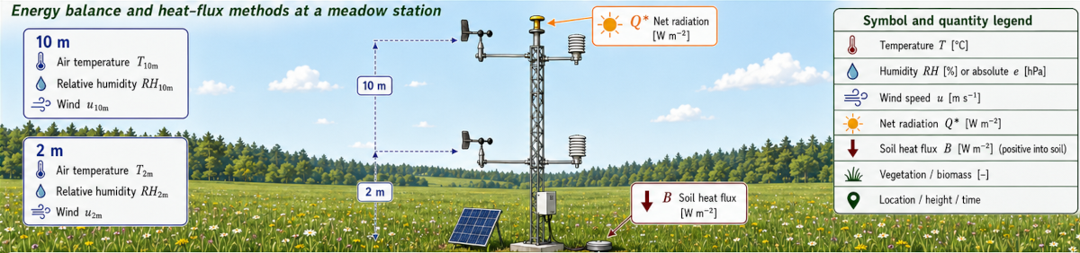
Surface energy balance and package sign convention
The common reference point is the reduced surface energy balance
without explicit storage or horizontal transport terms. This vignette
uses the same reference notation as the overview graphic and the
method-selection page: Q* is net radiation, B
is soil heat flux, A = Q* - B is available energy,
H is sensible heat flux, LE is latent heat
flux, and R_E is the residual or non-closed energy term.
The text deliberately avoids parallel notation such as
R_n/G or L/V in the main explanation. Package
internals and some Roxygen comments may use R_n and
G, but the tutorial and figure logic use Q*
and B consistently.
For readers without a meteorological background, the main idea is simple. Net radiation is the radiative energy gained or lost by the surface. Soil heat flux is the part of that energy that enters or leaves the ground. The remaining part is available for exchange with the air. Sensible heat changes air temperature. Latent heat is the energy involved in evaporation or condensation. The residual term collects what remains unresolved by a given method and dataset.
| Quantity | Reference notation | fieldClim field or output | Positive direction or meaning in fieldClim |
|---|---|---|---|
| Net radiation | Q* | rad_bal | net radiative energy input at the surface |
| Soil heat flux | B | soil_flux | heat flux into the soil |
| Available energy | A = Q* - B | rad_bal minus soil_flux | energy available for sensible and latent heat fluxes |
| Sensible heat flux | H | sensible_* | heat flux away from the surface |
| Latent heat flux | LE | latent_* | heat flux away from the surface |
| Residual / non-closed energy term | R_E = Q* - B - H - LE | closure_residual / unresolved_complement | remaining energy-balance difference |
The reduced available-energy definition is:
\[ A = Q^* - B \]
The diagnostic balance used throughout the documentation is:
\[ Q^* - B = H + LE + R_E \]
or equivalently:
\[ R_E = Q^* - B - H - LE \]
The package convention is: soil_flux is consumed as a
positive heat flux into the soil, while positive sensible and latent
heat fluxes are interpreted as fluxes away from the surface.
Overview graphic
A compact way to read the problem is this: the equation defines what should be accounted for, the flux family defines what is calculated first, and the closure regime describes how the resulting terms relate to available energy.

Energy accounting frame
The heat-flux methods operate inside a shared surface-energy accounting frame. This frame defines available energy and the residual term before any method-specific flux estimate is interpreted. Radiation and soil helpers belong to this input and accounting layer. They provide or model terms that all downstream method families depend on.
| Element | Role | Output / term | Interpretation rule |
|---|---|---|---|
| Master balance | defines the accounting frame | A, R_E | R_E is a composite residual term. It can contain measurement error, storage, advection, model mismatch, and unresolved exchange. |
| Radiation and soil helpers | provide or model input terms | Q, B, A = Q - B | Input consistency controls all downstream balances. Errors in Q* or B propagate into every method. |
This accounting layer is not a flux-estimation method. It supplies the frame within which flux families are interpreted.
Method classes
The methods belong to different micrometeorological method classes.
In fieldClim, these classes are implemented as distinct
calculation paths with different output semantics. The important
distinction is what each method estimates directly and what is then
derived, assigned, or left unresolved.
| Method class | Package method | Primary estimate | Package output logic |
|---|---|---|---|
| Available-energy evaporation method | Priestley–Taylor | LE from available energy and alpha | LE_PT, then H_PT = A - LE_PT |
| Bowen-ratio energy-balance method | Bowen ratio | H/LE partition from beta | H_BR and LE_BR from beta |
| Bulk-transfer method with residual closure | Bulk–Residual | H from temperature gradient and exchange assumption | H_bulk, then LE_res = A - H_bulk |
| Combination evaporation method | Penman / Penman-type | LE from available energy and atmospheric demand | LE_Penman; U_Penman = A - LE_Penman remains unresolved |
| Profile-gradient / similarity-based diagnostic | Monin–Obukhov / Profile | H and LE from profile/stability assumptions | H_MO, LE_MO; R_E,MO = A - H_MO - LE_MO remains visible |
Priestley-Taylor path
The Priestley-Taylor path estimates latent heat flux from available energy and an empirical coefficient (Priestley & Taylor, 1972). It is useful when the analysis needs an available-energy partition with relatively few profile assumptions.
\[ LE_{PT} = \alpha_{PT} \frac{\Delta}{\Delta + \gamma} (Q^* - B) \]
The corresponding sensible heat flux is the remaining available energy:
\[ H_{PT} = (Q^* - B) - LE_{PT} \]
Therefore the closure relation is:
\[ H_{PT} + LE_{PT} = Q^* - B \]
The method hides much of the surface-atmosphere coupling in
alpha_PT and in helper terms such as Delta and
gamma. In the package code, the slope term
Delta is stored as sc. The method provides an
interpretable partition of available energy rather than a direct
turbulent-flux measurement.
Bowen-ratio path
The Bowen-ratio method partitions available energy using the ratio of sensible to latent heat flux (bowen1926?; ohmura1982?):
\[ \beta = \frac{H}{LE} \]
If the ratio is known, the energy balance gives:
\[ H_{BR} = \frac{\beta}{1 + \beta} (Q^* - B) \]
and:
\[ LE_{BR} = \frac{1}{1 + \beta} (Q^* - B) \]
For finite uncapped denominators, the closure relation is:
\[ H_{BR} + LE_{BR} = Q^* - B \]
The implemented fieldClim Bowen ratio is based on a
potential-temperature gradient and an absolute-humidity gradient:
\[ \beta = \gamma_{code} \frac{\Delta \theta / \Delta z}{\Delta AH / \Delta z} \]
where:
\[ \gamma_{code} = 0.00066 (1 + 0.000946 t_1) \]
The implementation converts air temperature to potential temperature, converts relative humidity to absolute humidity, and then forms the gradient ratio. The Bowen path is physically meaningful when gradients are resolved and representative. Small humidity gradients, sign changes and near-zero denominator values can create very large fluxes. Numerical caps are safeguards, and capped cases should be treated as diagnostic rather than exact closure cases.
Bulk-Residual path
The Bulk-Residual path combines a wind- and temperature-gradient estimate of sensible heat flux with a residual latent heat flux. It is a station-data approximation in the aerodynamic-resistance family.
The sensible heat calculation follows:
\[ H_{bulk} = \rho c_p \frac{t_1 - t_2}{r_a} \]
A neutral resistance formulation is:
\[ r_a = \frac{\ln(z_2 / z_1)}{k\, velocity\_scale} \]
The current package default uses a wind-speed scale based on observed
wind speed. If two wind heights are available, the default uses the
arithmetic mean of v1 and v2; otherwise it
uses v1. A two-height station can also support a neutral
profile-derived friction velocity:
\[ u_* = k \frac{v_2 - v_1}{\ln(z_2 / z_1)} \]
and then:
\[ r_a = \frac{\ln(z_2 / z_1)}{k u_*} \]
This changes the exchange-velocity scale. Stability functions, Monin
length corrections and roughness sublayer effects are not applied to
H_bulk. The optional Richardson guard filters invalid or
very stable cases and leaves valid neutral fluxes unchanged.
The residual latent heat flux is:
\[ LE_{res} = Q^* - B - H_{bulk} \]
Therefore the Bulk-Residual workflow closes available energy by definition:
\[ H_{bulk} + LE_{res} = Q^* - B \]
This algebraic closure means that the residual latent heat flux
inherits all errors in Q*, B and the bulk
sensible heat estimate.
Penman-type latent heat path
The Penman family combines an energy term and an aerodynamic
vapour-pressure term (Allen et al., 1998; Penman,
1948). In fieldClim, latent_penman() is
a latent-heat method only. It returns no paired package-defined sensible
heat flux.
The package convention keeps the energy term as:
\[ Q^* - B \]
The simplified package interpretation is:
\[ LE_{Penman} = f(A, VPD, r_a, r_s) \]
Conceptually, Penman asks how much latent heat exchange is implied by radiation, atmospheric demand and resistance terms. The remaining available energy is unresolved within the Penman path.
\[ U_{Penman} = Q^* - B - LE_{Penman} \]
U_Penman may contain sensible heat, storage, advection,
input error and model mismatch. It should be reported as an unresolved
remainder rather than as H.
Monin-Obukhov and profile methods
Monin-Obukhov similarity theory and related profile-gradient methods attempt to represent turbulent transfer through vertical gradients, roughness, stability and surface-layer scaling (Foken, 2006; Stull, 1988; monin1954?). In package interpretation, the Monin/Profile path is a profile and stability diagnostic.
The diagnostic rule is:
\[ H_{MO} + LE_{MO} \]
is allowed to differ from:
\[ Q^* - B \]
The residual is:
\[ R_{E,MO} = Q^* - B - H_{MO} - LE_{MO} \]
A profile method estimates turbulent fluxes from profile and stability assumptions, while Priestley-Taylor, Bowen and Bulk-Residual are explicit energy-partition or residual workflows. The visible residual is therefore part of the diagnostic output.
The practical issue is numerical robustness. Zero gradients, very small wind shear, invalid height relationships and unstable stability functions can produce extreme outputs. Monin/Profile outputs should therefore be interpreted together with stability classification and diagnostic warnings. They should not be silently normalized to available energy.
Energy-balance closure as a modelling decision
The reduced balance is easy to write down, but it is not automatically observed in real field data. Radiation, soil heat flux, sensible heat and latent heat are not measured at exactly the same place, at the same effective footprint, with the same time response, or with the same uncertainty. In addition, energy may be stored in the air column, vegetation, biomass, water, litter or the upper soil layer. Energy may also be transported horizontally by advection or by coherent structures over heterogeneous terrain.
For this reason, R_E should be interpreted as a mixed
remainder. It may include storage, advection, dispersive transport,
footprint mismatch, measurement error, timing mismatch, parameterization
error and model error.
Different method families treat this remainder differently. They may use the same balance frame, but they do not give the same status to all terms. Some terms are measured or supplied as station inputs. Some are estimated by empirical or profile equations. Some are assumed by partitioning or residual definition. Some are left unresolved.
Direct flux measurements and closure literature
The closure interpretation in fieldClim connects to the
broader micrometeorological literature on surface energy balance
closure. This literature is important because it separates three things
that are easily confused: measured turbulent fluxes, available energy,
and the residual that remains between them.
Eddy-covariance systems estimate H and LE
directly from turbulent covariance data, but the sum of these turbulent
fluxes often does not equal Q* - B. Foken’s overview of the
energy-balance closure problem argues that non-closure cannot be reduced
to simple measurement error or storage alone; larger-scale exchange
processes over heterogeneous landscapes are central to the problem (Foken, 2008). Wilson et al. evaluated energy
balance closure across 22 FLUXNET sites and 50 site-years, showing that
closure is a network-scale issue rather than a local anomaly (Wilson et al., 2002). Leuning et al. describe
the surface energy imbalance problem as a mismatch between turbulent
fluxes and available energy, and discuss advective flux divergence and
related explanations (Leuning et al.,
2012). Mauder et al. revisit FLUXNET energy-balance closure and
treat closure as a continuing uncertainty for heat and water-vapour flux
assessments (Mauder et
al., 2024).
For non-meteorological readers, the implication is that energy-balance closure is not a simple pass/fail test. A closed method result can follow from the equations. An open result can be physically informative when it exposes storage, advection, footprint mismatch or model mismatch. The interpretation depends on the method family.
The closure types in fieldClim reflect this distinction.
Partition methods such as Priestley-Taylor and Bowen allocate available
energy within the reduced balance. Bulk-Residual assigns the latent flux
as the remaining available energy after H_bulk. Penman
leaves an unresolved remainder because it estimates only
LE. Monin/Profile keeps a diagnostic residual because its
fluxes are derived from profile and stability assumptions rather than
forced to equal available energy.
Closure regimes in fieldClim
Closure describes how method outputs relate to available energy. It is a consequence of the flux family and is not an additional flux method.
| Method | Closure regime | Unknown or residual term | Interpretation rule |
|---|---|---|---|
| Priestley-Taylor | partition closure | hidden in closure and empirical coefficient assumptions | Formal closure follows from the partitioning assumption and does not validate the physical split into H and LE. |
| Bowen ratio | partition closure for valid finite cases | hidden in ratio, gradient and denominator assumptions | Singular and capped cases require explicit filtering and must not be read as exact physical closure. |
| Bulk-Residual | residual closure by definition | LE_res is the assigned residual | Errors in Q*, B, or H_bulk enter the residual latent heat. |
| Penman / Penman-type | LE-only unresolved remainder | U_Penman remains unresolved | The complement remains unresolved and must not be labelled H. |
| Monin-Obukhov / Profile | profile diagnostic; not force-closed | R_E,MO remains visible | The residual remains visible and should be interpreted diagnostically. |
Partition closure
Priestley-Taylor and Bowen-ratio methods divide available energy into sensible and latent heat within the reduced balance:
\[ Q^* - B = H + LE \]
The method then decides how available energy is split between
H and LE. Priestley-Taylor uses an empirical
evaporation relation. Bowen uses a gradient-derived ratio between
sensible and latent heat. The hidden uncertainty lies in the empirical
coefficient, the gradient ratio, omitted storage and advection terms,
and the measurement/model inputs that define available energy.
Residual closure
Bulk-Residual first estimates sensible heat as H_bulk.
The remaining available energy is then assigned to latent heat:
\[ LE_{res} = Q^* - B - H_{bulk} \]
For finite and consistently computed fields, the closure residual is zero by definition:
\[ R_E = Q^* - B - H_{bulk} - LE_{res} = 0 \]
This is algebraic residual closure. It states how LE_res
was defined and therefore where errors in Q*,
B, or H_bulk enter the result.
LE-only unresolved remainder
Penman and Penman-type methods estimate latent heat. In
fieldClim, the Penman path does not provide a paired
package-defined sensible heat flux. The remaining term is:
\[ U_{Penman} = Q^* - B - LE_{Penman} \]
This term is an unresolved remainder. It may contain sensible heat, storage, advection, dispersive exchange, footprint mismatch and error terms.
Profile-diagnostic residual
Monin-Obukhov and profile methods estimate turbulent fluxes from profile, roughness and stability assumptions. They are not forced to close the available energy balance. Their residual is:
\[ R_{E,MO} = Q^* - B - H_{MO} - LE_{MO} \]
This residual shows whether the profile-based flux estimates, the radiation balance and the soil heat flux are mutually consistent. It should remain visible as a diagnostic output.
Canopy-layer and tower context
A tower or canopy setup is not just a question of sensor height above ground. The central question is which exchange layer is being interpreted: the under-canopy air space, the within-canopy layer, the canopy-top transition, or the above-canopy layer. A sensor pair inside the canopy, across the canopy top, or above the canopy represents different physical processes.
If one relevant height is used, the result mainly describes the local microclimate and available-energy state at that level. If two relevant heights are used, Bulk-Residual, Bowen, or Monin/Profile diagnostics can be used only after the height pair has been assigned to a canopy-layer interpretation. The result should then be reported as exchange or coupling diagnostics, not as a generic surface-layer flux.
| Canopy / tower situation | First decision | Method role | Reportable finding |
|---|---|---|---|
| One height near forest floor or below canopy | define local ground or under-canopy context | Penman, Priestley-Taylor, available-energy diagnostics if Q* and B fit that context | local under-canopy energy context |
| One height within canopy | define local within-canopy context | Penman, Priestley-Taylor, available-energy diagnostics if Q* and B fit that context | local within-canopy energy context |
| Two heights within canopy | define whether the target is vertical coupling inside the canopy | diagnostic only; Bulk/Bowen only with caution | within-canopy coupling or decoupling signal |
| One height within canopy and one height above canopy | define whether the target is canopy-top exchange | Bulk-Residual, Bowen, or Monin/Profile only with explicit height and roughness logic | canopy-top exchange diagnostic |
| Two heights above canopy | define the above-canopy reference layer | Bulk-Residual, Bowen, or Monin/Profile diagnostic | above-canopy exchange comparison |
| Unknown canopy-layer context | do not force flux interpretation | exploratory diagnostics only | flux interpretation remains underdefined |
Practical interpretation in fieldClim
The methods should be read as complementary diagnostics rather than as competitors in a single accuracy ranking.
Priestley-Taylor partitions available energy through an empirical latent-heat formulation. Bulk-Residual estimates sensible heat from a two-height gradient and defines latent heat as the residual. Bowen partitions available energy through temperature and humidity gradients. Penman estimates latent heat and leaves the remaining energy unresolved. Monin/Profile provides a profile- and stability-oriented diagnostic and keeps the residual visible.
A robust package summary is therefore:
fieldClimimplements common micrometeorological approximation families for heat-flux analysis from weather-station data. Priestley-Taylor, Bowen-ratio, Penman-type, bulk-resistance/residual and Monin-Obukhov/profile methods differ in data requirements and assumptions. Some methods close the available energy by partition or by residual definition; others are latent-heat-only or diagnostic profile estimates. Formal closure describes method semantics and open residuals can be diagnostically meaningful.