fieldClim: Follow-up workflows and additional package functions

Aim of this vignette

This vignette complements the energy-balance workflow vignette. That vignette focuses on the coherent Caldern workflow with \(Q^{*}\), \(B\), \(H\), and \(LE\). This page presents the additional package functions as follow-up workflows: radiation checks, modelled radiation, soil parameters, meteorological helper variables, stability variables, and object control.

A systematic decision guide for matching heat-flux methods to measurement architecture is provided in Choosing fieldClim Heat-Flux Methods by Measurement Design. This vignette applies that logic to the follow-up workflows around the Caldern example dataset.

The text is not a second comparison of methods. The central question here is: Which groups of functions exist beyond the main workflow, what are they practically useful for, and which limitations must be considered when applying them?

Module	Guiding question	Package area
0	How does the package work in general?	`weather_station`, default methods, S3 methods
1	How can radiation time series be checked without silently replacing measurements?	`rad_*`, measurement columns, time-series checks
2	How can radiation be modelled when measurements are missing or when a plausibility benchmark is needed?	`sol_`, `trans_`, `terr_`, `rad_`
3	How are soil parameters and soil heat flux handled?	`soil_*`
4	Which helper variables are needed for humidity, pressure, and temperature?	`hum_`, `pres_`, `temp_*`
5	How are the wind profile, Richardson number, and stability variables checked?	`turb_`, `bound_` as diagnostic follow-up functions
6	How is a `weather_station` object checked, plotted, and exported?	`build_weather_station()`, `plot_weather_station()`, `as.data.frame()`

This vignette is a package map with executable mini examples. It does not replace a complete physical derivation, nor does it provide testing against independent flux measurements. Its purpose is to show which package functions fit which workflow steps.

Reference notation and code variables

This vignette uses the reference notation from the method-selection page. Q* is net radiation, B is soil heat flux, A = Q* - B is available energy, H is sensible heat flux, LE is latent heat flux, and R_E is the residual or non-closed energy term.

Longwave radiation is kept separate from turbulent heat flux notation. L_down, L_up, and L* refer to longwave radiation components. This L is not sensible heat flux. Sensible heat flux is denoted as H.

The R code variables used in this tutorial are not renamed. Existing objects such as L_monin_no_cap, V_bowen_no_cap, or other L_* and V_* objects are kept because they belong to the current tutorial workflow. In the explanatory text, however, L_* is interpreted as H, and V_* is interpreted as LE.

Reference quantity	Meaning	`fieldClim` field or output	Tutorial code variable
`Q*`	net radiation	`rad_bal`	`Q_star`
`B`	soil heat flux	`soil_flux`	`B`, `B_measured`, `B_model`
`A = Q* - B`	available energy	`rad_bal - soil_flux`	`available_energy`, `Q_minus_B`
`H`	sensible heat flux	`sensible_*`	`L_*` where used as tutorial working variable
`LE`	latent heat flux	`latent_*`	`V_*` where used as tutorial working variable
`R_E = Q* - B - H - LE`	residual / non-closed energy term	closure diagnostic output	`closure_residual`, `diff_*`

Shared data and object setup

All modules use the same small teaching dataset. The dataset is included in the installed package under inst/extdata/.

# Load fieldClim.
library(fieldClim)

# Path to the included teaching file.
caldern_file <- system.file(
  "extdata",
  "caldern_wiese_2017-06-30.csv",
  package = "fieldClim"
)

# Read the CSV file.
# "NULL", "NA", and empty entries are treated as missing values.
caldern <- read.csv(
  caldern_file,
  na.strings = c("NULL", "NA", "")
)

# Interpret timestamps explicitly as local station time.
caldern$datetime <- as.POSIXct(
  caldern$datetime,
  format = "%Y-%m-%d %H:%M:%S",
  tz = "Europe/Berlin"
)

# The solar and radiation functions can work with POSIXct timestamps.
# The time zone therefore remains explicitly set.
# Basic checks.
nrow(caldern)
#> [1] 288
range(caldern$datetime)
#> [1] "2017-06-30 00:00:00 CEST" "2017-06-30 23:55:00 CEST"
summary(diff(caldern$datetime))
#> Time differences in mins
#>    Min. 1st Qu.  Median    Mean 3rd Qu.    Max. 
#>       5       5       5       5       5       5
names(caldern)
#>  [1] "record"         "datetime"       "Ta_2m"          "Huma_2m"       
#>  [5] "Ta_10m"         "Huma_10m"       "Windspeed_2m"   "Windspeed_10m" 
#>  [9] "rad_sw_in"      "rad_sw_out"     "RsNet"          "RlNet"         
#> [13] "rad_net"        "LUpCo"          "LDnCo"          "water_vol_soil"
#> [17] "Ts"             "heatflux_soil"  "PCP"

# A weather_station object combines measurements, location, and model assumptions.
# This object can be passed to many package functions.
ws <- build_weather_station(
  datetime = caldern$datetime,
  lon = 8.6832,
  lat = 50.8405,
  elev = 261,

  temp = caldern$Ta_2m,
  rh = caldern$Huma_2m,

  t1 = caldern$Ta_2m,
  t2 = caldern$Ta_10m,
  hum1 = caldern$Huma_2m,
  hum2 = caldern$Huma_10m,

  v1 = caldern$Windspeed_2m,
  v2 = caldern$Windspeed_10m,
  z1 = 2,
  z2 = 10,

  slope = 0,
  exposition = 0,
  valley = FALSE,

  surface_type = "field",
  # surface_temp is an explicit model input for radiation functions, not an
  # automatically available standard station measurement.
  surface_temp = caldern$Ts,

  texture = "peat",
  moisture = caldern$water_vol_soil,

  rad_bal = caldern$rad_net,
  soil_flux = caldern$heatflux_soil,

  soil_temp1 = caldern$Ts,
  soil_temp2 = caldern$Ta_2m,
  soil_depth1 = 0.25,
  soil_depth2 = 0,

  obs_height = 2
)

class(ws)
#> [1] "weather_station"
names(ws)
#>  [1] "datetime"     "lon"          "lat"          "elev"         "temp"        
#>  [6] "rh"           "t1"           "t2"           "hum1"         "hum2"        
#> [11] "v1"           "v2"           "z1"           "z2"           "slope"       
#> [16] "exposition"   "valley"       "surface_type" "surface_temp" "texture"     
#> [21] "moisture"     "rad_bal"      "soil_flux"    "soil_temp1"   "soil_temp2"  
#> [26] "soil_depth1"  "soil_depth2"  "obs_height"

Interpretation. The weather_station object is the central working container of the package. Many functions have two usage forms: a default method with individual arguments and a method for weather_station. The object-based route is useful as soon as several functions need the same measurements, site data, and surface assumptions.

Workflow module 0: Default method or weather_station method?

Almost every central function can be used directly with individual arguments or with a weather_station object.

# Default method: all required arguments are provided individually.
pres_p(elev = 261, temp = 20)
#> [1] 982.884

# Object method: the function reads the required variables from the weather_station object.
pres_p(ws)
#>   [1] 982.1623 982.1537 982.1548 982.1697 982.1815 982.2263 982.2327 982.2220
#>   [9] 982.2178 982.2295 982.2210 982.2146 982.2114 982.2050 982.2007 982.2007
#>  [17] 982.2018 982.2007 982.2007 982.2018 982.2007 982.2007 982.2018 982.1964
#>  [25] 982.1954 982.1932 982.1879 982.1772 982.1644 982.1537 982.1419 982.1419
#>  [33] 982.1366 982.1376 982.1387 982.1398 982.1344 982.1269 982.1205 982.1119
#>  [41] 982.1066 982.1044 982.1066 982.1098 982.1109 982.1141 982.1141 982.1141
#>  [49] 982.1162 982.1184 982.1194 982.1216 982.1280 982.1312 982.1366 982.1398
#>  [57] 982.1409 982.1473 982.1526 982.1623 982.1719 982.1815 982.1932 982.2039
#>  [65] 982.2135 982.2092 982.2242 982.2295 982.2401 982.2561 982.2667 982.2773
#>  [73] 982.2837 982.2858 982.2869 982.2816 982.2762 982.2741 982.2752 982.2890
#>  [81] 982.2953 982.3123 982.3282 982.3313 982.3430 982.3630 982.3884 982.3989
#>  [89] 982.4042 982.3968 982.3768 982.3841 982.3936 982.4052 982.4367 982.4913
#>  [97] 982.4976 982.5028 982.4965 982.4913 982.4986 982.4944 982.5331 982.5810
#> [105] 982.5706 982.6091 982.6029 982.5821 982.5800 982.5633 982.5581 982.5696
#> [113] 982.5831 982.5873 982.5779 982.5456 982.5456 982.5706 982.6049 982.5935
#> [121] 982.5800 982.6382 982.7198 982.7033 982.6723 982.6785 982.6961 982.7302
#> [129] 982.7363 982.7857 982.7744 982.7322 982.7353 982.7785 982.8001 982.7908
#> [137] 982.7775 982.7867 982.7878 982.8083 982.7785 982.7734 982.7775 982.7291
#> [145] 982.7219 982.7353 982.7672 982.7919 982.7775 982.7867 982.8001 982.8308
#> [153] 982.8594 982.8154 982.7939 982.7816 982.7549 982.7435 982.7621 982.7785
#> [161] 982.7713 982.7580 982.7590 982.7641 982.8031 982.8144 982.8083 982.8329
#> [169] 982.8972 982.8451 982.8165 982.8236 982.8062 982.7888 982.7723 982.7672
#> [177] 982.7662 982.7723 982.7929 982.7898 982.7990 982.7929 982.7939 982.8103
#> [185] 982.8206 982.8206 982.8144 982.8175 982.8247 982.8380 982.8809 982.8727
#> [193] 982.8829 982.8809 982.8850 982.8809 982.8707 982.8431 982.8195 982.8195
#> [201] 982.8277 982.8144 982.8021 982.7990 982.7888 982.7878 982.7713 982.7528
#> [209] 982.7785 982.7919 982.7929 982.7908 982.7898 982.7734 982.7631 982.7580
#> [217] 982.7281 982.7085 982.6837 982.6858 982.6485 982.6101 982.5956 982.5633
#> [225] 982.5362 982.5070 982.4923 982.5059 982.4766 982.4493 982.4504 982.4420
#> [233] 982.4157 982.4031 982.3789 982.3546 982.3282 982.3049 982.3123 982.3038
#> [241] 982.3102 982.2816 982.2656 982.2454 982.2359 982.2199 982.2082 982.1975
#> [249] 982.2039 982.2071 982.2103 982.2071 982.2039 982.1847 982.1719 982.1815
#> [257] 982.1665 982.1484 982.1430 982.1344 982.1184 982.1055 982.0969 982.0990
#> [265] 982.0958 982.0915 982.0883 982.0915 982.0969 982.0990 982.0872 982.0872
#> [273] 982.0905 982.0851 982.0765 982.0786 982.0743 982.0711 982.0636 982.0636
#> [281] 982.0571 982.0539 982.0560 982.0560 982.0604 982.0582 982.0571 982.0636

Interpretation. The default method is useful for individual tests and for tracing formulas. The weather_station method is better for workflows because it carries the same data structure through several calculation steps.

Workflow module 1: Check radiation time series and define the working variable

Radiation time series are often the most important input for energy-balance calculations. Before \(Q^{*}\) is used as net radiation, the components must be checked.

The shortwave balance is:

\[ K^{*} = K_{\downarrow} - K_{\uparrow} \]

with:

\(K^{*}\): shortwave balance [W/m²]
\(K_{\downarrow}\): incoming shortwave radiation [W/m²]
\(K_{\uparrow}\): reflected shortwave radiation [W/m²]

The longwave balance is written here in the same direction:

\[ L^{*} = L_{\downarrow} - L_{\uparrow} \]

with:

\(L^{*}\): longwave balance [W/m²]
\(L_{\downarrow}\): incoming longwave radiation [W/m²]
\(L_{\uparrow}\): longwave emission from the surface [W/m²]

Here, L denotes longwave radiation. It does not denote sensible heat flux; sensible heat is denoted as H in the reference notation used in this vignette.

The net radiation is theoretically given by:

\[ Q^{*} = K^{*} + L^{*} \]

with:

\(Q^{*}\): net radiation or radiation balance [W/m²]

1.1 Calculate components and compare them with stored net columns

# Shortwave components from measurement columns.
caldern$K_down <- caldern$rad_sw_in
caldern$K_up <- caldern$rad_sw_out
caldern$K_star_from_components <- caldern$K_down - caldern$K_up

# Longwave components from measurement columns.
caldern$L_down <- caldern$LDnCo
caldern$L_up <- caldern$LUpCo
caldern$L_star_down_minus_up <- caldern$L_down - caldern$L_up
caldern$L_star_up_minus_down <- caldern$L_up - caldern$L_down

# Check against existing net columns.
shortwave_check <- summary(caldern$K_star_from_components - caldern$RsNet)
longwave_check_down_up <- summary(caldern$L_star_down_minus_up - caldern$RlNet)
longwave_check_up_down <- summary(caldern$L_star_up_minus_down - caldern$RlNet)

shortwave_check
#>      Min.   1st Qu.    Median      Mean   3rd Qu.      Max. 
#> -0.400000  0.000000  0.000000  0.004208  0.001000  0.500000
longwave_check_down_up
#>    Min. 1st Qu.  Median    Mean 3rd Qu.    Max. 
#>   3.595  32.337  78.015  74.076 100.468 187.400
longwave_check_up_down
#>      Min.   1st Qu.    Median      Mean   3rd Qu.      Max. 
#> -0.090000 -0.030000  0.000000 -0.001698  0.030000  0.100000

Interpretation. This step checks which column definition is consistent. If rad_sw_in - rad_sw_out matches RsNet well, the shortwave balance is clear. For the longwave balance, the sign direction must be checked. Depending on whether LDnCo - LUpCo or LUpCo - LDnCo matches RlNet better, a different convention is present.

1.2 Check net radiation from net columns and individual components

# Variant A: net radiation from stored net columns.
caldern$Q_star_from_net_columns <- caldern$RsNet + caldern$RlNet

# Variant B: net radiation from individual components.
caldern$Q_star_from_components <- caldern$K_star_from_components +
  caldern$L_star_down_minus_up

# Existing net radiation.
caldern$Q_star_measured <- caldern$rad_net

# Check differences.
summary(caldern$Q_star_from_net_columns - caldern$Q_star_measured)
#>      Min.   1st Qu.    Median      Mean   3rd Qu.      Max. 
#> -0.100000 -0.010000  0.000000 -0.002542  0.005000  0.100000
summary(caldern$Q_star_from_components - caldern$Q_star_measured)
#>    Min. 1st Qu.  Median    Mean 3rd Qu.    Max. 
#>   3.595  32.331  78.013  74.078 100.515 187.700

op <- par(mfrow = c(2, 1), mar = c(3.5, 4, 2, 1))

plot(
  caldern$datetime,
  caldern$Q_star_measured,
  type = "l",
  col = "#000000",
  lwd = 2,
  xlab = "Time",
  ylab = "W/m²",
  main = "Q*: existing net radiation"
)

lines(caldern$datetime, caldern$Q_star_from_net_columns, col = "#0072B2", lwd = 2)

legend(
  "bottomleft",
  legend = c("rad_net", "RsNet + RlNet"),
  col = c("#000000", "#0072B2"),
  lty = 1,
  lwd = 2,
  bty = "n"
)

plot(
  caldern$Q_star_measured,
  caldern$Q_star_from_components,
  pch = 16,
  col = rgb(0, 0, 0, 0.35),
  xlab = "rad_net [W/m²]",
  ylab = "K* + L* from individual components [W/m²]",
  main = "Compatibility check of radiation columns"
)

abline(0, 1, lty = 2, col = "grey40")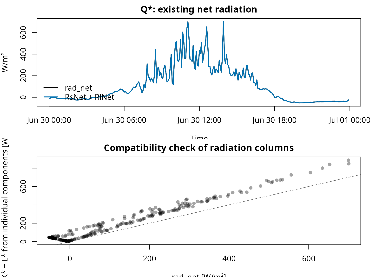


par(op)

Interpretation. This module is a data-check workflow. The package functions can only be used meaningfully when it is clear which radiation variable is used as the working variable. If rad_net, RsNet + RlNet, and K* + L* diverge, a new net radiation series is not created automatically. Instead, the first step is to document which column represents which balance level.

1.3 Define the radiation time series for further calculations

# Working decision:
# For energy-balance workflows, the existing rad_net column is used.
# The other variants remain diagnostic variables.
caldern$Q_star <- caldern$Q_star_measured

# Document summary statistics of the differences.
radiation_decision <- data.frame(
  Comparison = c(
    "RsNet + RlNet against rad_net",
    "K* + L* against rad_net"
  ),
  Mean_deviation = c(
    mean(caldern$Q_star_from_net_columns - caldern$Q_star_measured, na.rm = TRUE),
    mean(caldern$Q_star_from_components - caldern$Q_star_measured, na.rm = TRUE)
  ),
  Max_abs_deviation = c(
    max(abs(caldern$Q_star_from_net_columns - caldern$Q_star_measured), na.rm = TRUE),
    max(abs(caldern$Q_star_from_components - caldern$Q_star_measured), na.rm = TRUE)
  )
)

radiation_decision[, -1] <- round(radiation_decision[, -1], 1)
radiation_decision
#>                      Comparison Mean_deviation Max_abs_deviation
#> 1 RsNet + RlNet against rad_net            0.0               0.1
#> 2       K* + L* against rad_net           74.1             187.7

Interpretation. This is the actual “fix”: do not silently overwrite values, but define a working series and keep the alternatives as diagnostic variables. When heat fluxes are calculated later, it remains transparent which version of \(Q^{*}\) was used.

1.4 Check time lag

A time lag of one 5-minute step can create large deviations in radiation data.

# Mean absolute deviation without lag.
diff_0 <- mean(abs(
  caldern$Q_star_from_components - caldern$Q_star_measured
), na.rm = TRUE)

# Compare the component sum one step later against rad_net.
diff_plus <- mean(abs(
  caldern$Q_star_from_components[-1] -
    caldern$Q_star_measured[-length(caldern$Q_star_measured)]
), na.rm = TRUE)

# Compare the component sum one step earlier against rad_net.
diff_minus <- mean(abs(
  caldern$Q_star_from_components[-length(caldern$Q_star_from_components)] -
    caldern$Q_star_measured[-1]
), na.rm = TRUE)

lag_check <- data.frame(
  Comparison = c(
    "without lag",
    "components +1 step",
    "components -1 step"
  ),
  mean_absolute_deviation = c(diff_0, diff_plus, diff_minus)
)

lag_check$mean_absolute_deviation <- round(
  lag_check$mean_absolute_deviation,
  1
)

lag_check
#>           Comparison mean_absolute_deviation
#> 1        without lag                    74.1
#> 2 components +1 step                    83.4
#> 3 components -1 step                    85.8

Interpretation. If a shifted comparison becomes clearly better, a timestamp or aggregation problem is likely. If it does not improve, this points more toward different column definitions, correction levels, or sign conventions.

Workflow module 2: Model radiation instead of only measuring it

The radiation functions can be used to check the plausibility of measurements or to model missing radiation components. The package calculation logic follows a chain:

Subproblem	Function family	Role
Solar position	`sol_*`	Day angle, solar elevation, azimuth
Atmospheric attenuation	`trans_*`	Air mass, gas, ozone, Rayleigh, water-vapour, and aerosol transmission
Terrain	`terr_*`	Terrain and sky-view geometry
Radiation	`rad_*`	Shortwave, diffuse, longwave, and net radiation

# Example timestamp for an individual test.
# POSIXct is deliberately retained here; the current package version handles
# POSIXct/POSIXlt consistently.
example_time <- as.POSIXct("2017-06-30 12:00:00", tz = "Europe/Berlin")

# Location and assumptions.
lon <- 8.6832
lat <- 50.8405
elev <- 261
temp <- 20
rh <- 60
slope <- 0
exposition <- 0
valley <- FALSE
surface_type <- "field"
# Explicit model input for longwave radiation; not a standard station sensor.
surface_temp <- 20

# Solar and topographic partial variables.
sol_elevation(example_time, lon, lat)
#> [1] 62.36272
sol_azimuth(example_time, lon, lat)
#> [1] 181.1272
terr_sky_view(slope, valley)
#> [1] 1

# Modelled shortwave and longwave radiation.
rad_sw_in(example_time, lon, lat, elev, temp, slope, exposition)
#> [1] 704.2516
rad_sw_bal(example_time, lon, lat, elev, temp, slope, exposition, valley, surface_type)
#> [1] 673.2495
rad_lw_bal(temp, rh, slope, valley, surface_type, surface_temp)
#> [1] -105.0535

# Modelled net radiation. This also uses Ts as explicit surface-temperature input.
rad_bal(
  example_time, lon, lat, elev, temp, rh,
  slope, exposition, valley, surface_type, surface_temp
)
#> [1] 568.196

Interpretation. This module is relevant when radiation components are missing or when measurements need to be checked against a plausible order of magnitude. Modelled radiation is not an automatic replacement measurement here. It is a benchmark: if the diurnal cycle and magnitude roughly agree, this supports a consistent time basis and realistic site assumptions. If measurement and model diverge strongly, the first checks should address time zone, surface type, terrain parameters, sensor processing, or differently defined radiation components. The time basis is technically important here: the current package version handles POSIXct and POSIXlt timestamps consistently. The key point remains that the time zone must be set explicitly because solar position and radiation depend on local time. surface_temp is used here only as an explicit model input for longwave radiation. It is not treated as a standard automatically available station sensor.

2.1 Compare measured and modelled radiation as a diurnal cycle

# Modelled incoming shortwave radiation for the full teaching day.
# The function is vectorised over the POSIXct time axis.
caldern$K_down_model <- rad_sw_in(
  caldern$datetime,
  lon, lat, elev, caldern$Ta_2m,
  slope, exposition
)

# Modelled shortwave balance.
caldern$K_star_model <- rad_sw_bal(
  caldern$datetime,
  lon, lat, elev, caldern$Ta_2m,
  slope, exposition, valley, surface_type
)

# Modelled longwave balance. This uses Ts as explicit surface-temperature input.
caldern$L_star_model <- rad_lw_bal(
  caldern$Ta_2m,
  caldern$Huma_2m,
  slope,
  valley,
  surface_type,
  caldern$Ts
)

# Modelled net radiation. This also uses Ts as explicit surface-temperature input.
caldern$Q_star_model <- rad_bal(
  caldern$datetime,
  lon, lat, elev, caldern$Ta_2m, caldern$Huma_2m,
  slope, exposition, valley, surface_type, caldern$Ts
)

op <- par(mfrow = c(3, 1), mar = c(3.5, 4, 2, 1))

plot(
  caldern$datetime,
  caldern$K_down,
  type = "l",
  col = "#000000",
  lwd = 2,
  xlab = "Time",
  ylab = "W/m²",
  main = "Incoming shortwave radiation: measurement and model"
)
lines(caldern$datetime, caldern$K_down_model, col = "#D55E00", lwd = 2)
legend(
  "topright",
  legend = c("measured", "modelled"),
  col = c("#000000", "#D55E00"),
  lty = 1,
  lwd = 2,
  bty = "n"
)

plot(
  caldern$datetime,
  caldern$Q_star,
  type = "l",
  col = "#000000",
  lwd = 2,
  xlab = "Time",
  ylab = "W/m²",
  main = "Net radiation: working series and model"
)
lines(caldern$datetime, caldern$Q_star_model, col = "#0072B2", lwd = 2)

plot(
  caldern$Q_star,
  caldern$Q_star_model,
  pch = 16,
  col = rgb(0, 0, 0, 0.35),
  xlab = "Q* working series [W/m²]",
  ylab = "Q* modelled [W/m²]",
  main = "Radiation model as plausibility check"
)
abline(0, 1, lty = 2, col = "grey40")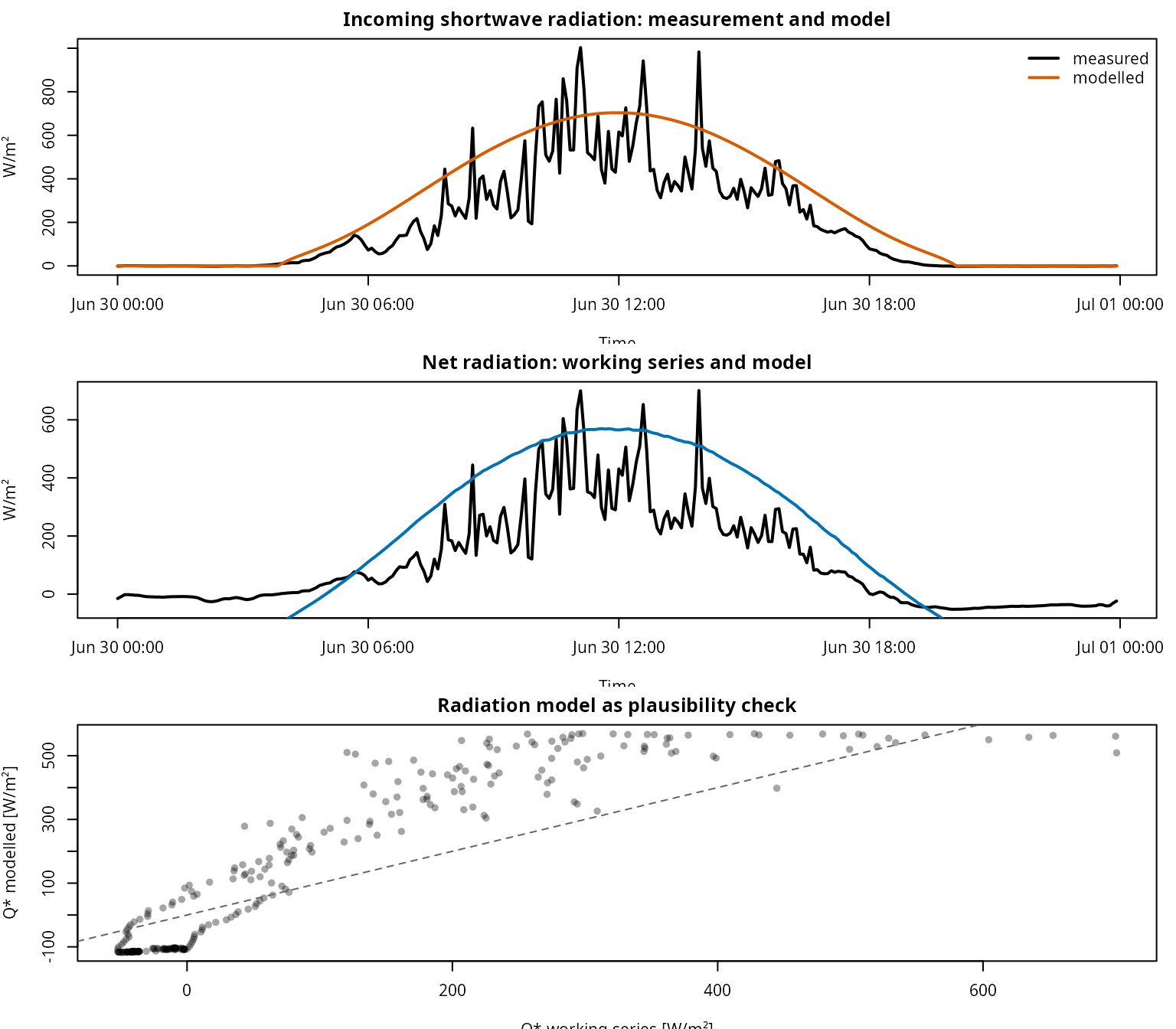


par(op)

Interpretation. Modelled radiation does not automatically replace measurement. It helps identify whether measurement series are temporally plausible and whether terrain, surface, or transmission assumptions produce realistic orders of magnitude.

Workflow module 3: Soil parameters and soil heat flux

Soil heat flux can be measured or estimated from the temperature gradient, depth, moisture, and soil texture. The package calculation logic is:

\[ B = -\lambda_s \frac{T_1 - T_2}{z_1 - z_2} \]

with:

\(B\): soil heat flux [W/m²]
\(\lambda_s\): soil thermal conductivity [W/(m K)]
\(T_1\): soil temperature at depth \(z_1\) [°C or K]
\(T_2\): temperature at the second depth or at the surface \(z_2\) [°C or K]
\(z_1\): depth of the first sensor [m]
\(z_2\): depth of the second reference [m]

# Thermal conductivity for the selected soil texture and moisture.
soil_thermal_cond(texture = "peat", moisture = mean(caldern$water_vol_soil, na.rm = TRUE))
#> [1] 0.1634507

# Soil heat flux from the weather_station object.
caldern$B_model <- soil_heat_flux(ws)

# Measured working variable.
caldern$B_measured <- caldern$heatflux_soil

summary(caldern$B_model - caldern$B_measured)
#>    Min. 1st Qu.  Median    Mean 3rd Qu.    Max. 
#> -7.0809 -5.4063 -2.9097 -3.1374 -0.9378  0.7452

op <- par(mfrow = c(2, 1), mar = c(3.5, 4, 2, 1))

plot(
  caldern$datetime,
  caldern$B_measured,
  type = "l",
  col = "#000000",
  lwd = 2,
  xlab = "Time",
  ylab = "W/m²",
  main = "Soil heat flux: measured"
)

plot(
  caldern$datetime,
  caldern$B_model,
  type = "l",
  col = "#009E73",
  lwd = 2,
  xlab = "Time",
  ylab = "W/m²",
  main = "Soil heat flux: calculated from soil parameters"
)


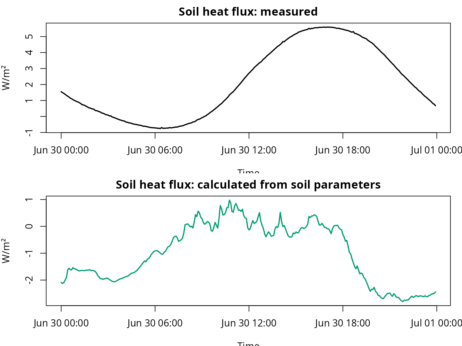
par(op)

Interpretation. The soil module is mainly useful in two situations: either directly measured soil heat flux is missing, or soil moisture and texture are to be varied as scenarios. However, a value calculated from a temperature gradient and soil parameters is not the same as a heat-flux plate measurement. Differences are therefore expected. For the energy balance, it is important to preserve the sign convention: in fieldClim, positive soil_flux means that heat enters the soil and is therefore subtracted from the available turbulent energy.

Workflow module 4: Humidity, pressure, and temperature as helper variables

Humidity, pressure, and temperature functions are usually not end products. They provide intermediate variables for radiation, stability, and heat-flux methods.

# Absolute humidity from relative humidity and temperature.
caldern$hum_abs <- hum_absolute(caldern$Huma_2m, caldern$Ta_2m)

# Latent heat of vaporisation as a temperature-dependent helper variable.
caldern$evap_heat <- hum_evap_heat(caldern$Ta_2m)

# Humidity gradient between two measurement heights.
caldern$hum_gradient <- hum_moisture_gradient(
  caldern$Huma_2m,
  caldern$Huma_10m,
  caldern$Ta_2m,
  caldern$Ta_10m,
  2,
  10,
  261
)

# Air density from elevation and temperature.
caldern$air_density <- pres_air_density(261, caldern$Ta_2m)

# Potential temperature.
caldern$theta <- temp_pot_temp(caldern$Ta_2m, 261)

summary(caldern[, c("hum_abs", "evap_heat", "hum_gradient", "air_density", "theta")])
#>     hum_abs           evap_heat        hum_gradient         air_density   
#>  Min.   :0.009325   Min.   :2453052   Min.   :-1.384e-04   Min.   :1.168  
#>  1st Qu.:0.010098   1st Qu.:2456082   1st Qu.:-5.213e-05   1st Qu.:1.172  
#>  Median :0.010462   Median :2464544   Median :-3.834e-05   Median :1.187  
#>  Mean   :0.010676   Mean   :2463389   Mean   :-3.671e-05   Mean   :1.185  
#>  3rd Qu.:0.011350   3rd Qu.:2469324   3rd Qu.:-2.394e-05   3rd Qu.:1.195  
#>  Max.   :0.011986   Max.   :2472146   Max.   : 1.735e-05   Max.   :1.199  
#>      theta      
#>  Min.   :13.56  
#>  1st Qu.:14.75  
#>  Median :16.75  
#>  Mean   :17.24  
#>  3rd Qu.:20.31  
#>  Max.   :21.58

op <- par(mfrow = c(2, 1), mar = c(3.5, 4, 2, 1))

plot(
  caldern$datetime,
  caldern$hum_abs,
  type = "l",
  col = "#0072B2",
  lwd = 2,
  xlab = "Time",
  ylab = "kg/kg or package-internal unit",
  main = "Absolute humidity"
)

plot(
  caldern$datetime,
  caldern$air_density,
  type = "l",
  col = "#D55E00",
  lwd = 2,
  xlab = "Time",
  ylab = "kg/m³",
  main = "Air density"
)


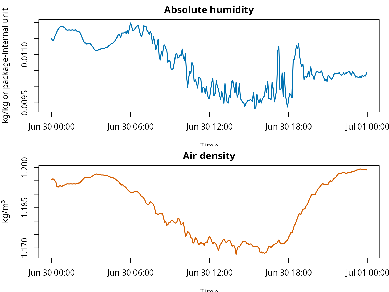
par(op)

Interpretation. These helper variables are intermediate steps, not independent result fluxes. Absolute humidity, potential temperature, air density, and latent heat of vaporisation later enter gradient analyses, Bowen, Penman, and profile-related calculation paths. This is exactly why they matter: a small unit or scaling error in a helper variable can later appear as a large difference in heat flux.

Workflow module 5: Wind profile, Richardson number, and stability

Before using profile-related heat-flux calculation paths, the wind profile, roughness, and stability should be checked. The package provides several turb_* functions for this purpose.

# Roughness length from the surface type.
z0 <- turb_roughness_length("field")
z0
#> [1] 0.02

# Friction velocity from wind speed and measurement height.
caldern$u_star <- turb_ustar(caldern$Windspeed_2m, 2, surface_type = "field")

# Gradient Richardson number.
caldern$richardson <- turb_flux_grad_rich_no(
  caldern$Ta_2m,
  caldern$Ta_10m,
  2,
  10,
  caldern$Windspeed_2m,
  caldern$Windspeed_10m,
  261
)

# Exchange and stability variables from the package.
caldern$exchange_temp <- turb_flux_ex_quotient_temp(
  caldern$Ta_2m,
  caldern$Ta_10m,
  2,
  10,
  caldern$Windspeed_2m,
  caldern$Windspeed_10m,
  261,
  "field"
)

summary(caldern[, c("u_star", "richardson", "exchange_temp")])
#>      u_star          richardson        exchange_temp      
#>  Min.   :0.01216   Min.   :-2389.420   Min.   : 0.007292  
#>  1st Qu.:0.04271   1st Qu.:   -0.398   1st Qu.: 0.020282  
#>  Median :0.05959   Median :    1.346   Median : 0.029678  
#>  Mean   :0.06898   Mean   :  265.130   Mean   : 0.301201  
#>  3rd Qu.:0.09205   3rd Qu.:    7.225   3rd Qu.: 0.259571  
#>  Max.   :0.16998   Max.   :67806.240   Max.   :14.292973

op <- par(mfrow = c(3, 1), mar = c(3.5, 4, 2, 1))

plot(
  caldern$datetime,
  caldern$u_star,
  type = "l",
  col = "#000000",
  lwd = 2,
  xlab = "Time",
  ylab = "m/s",
  main = "u*: friction velocity"
)

plot(
  caldern$datetime,
  caldern$richardson,
  type = "l",
  col = "#D55E00",
  lwd = 2,
  xlab = "Time",
  ylab = "Ri",
  main = "Gradient Richardson number"
)
abline(h = 0, lty = 2, col = "grey50")

plot(
  caldern$datetime,
  caldern$exchange_temp,
  type = "l",
  col = "#0072B2",
  lwd = 2,
  xlab = "Time",
  ylab = "Exchange coefficient",
  main = "Temperature exchange diagnostics"
)


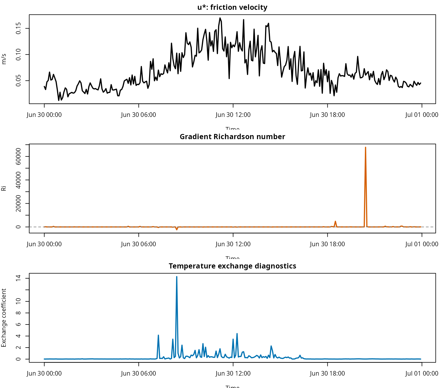
par(op)

Interpretation. This module checks whether the profile information is usable at all. Richardson number and exchange variables depend on temperature differences, wind-speed differences, and measurement heights. If wind shear is very small or signs change, stability statements become sensitive. These are exactly the situations that later explain why profile-based heat-flux values can become conspicuous. The values should therefore first be read as plausibility and screening variables, not as an energy balance of their own.

5.1 Document protection parameters and critical edge cases

Some methods have cap arguments or return NA in a controlled way for invalid cases. These protection mechanisms are not a physical solution. They mark or limit situations in which denominators are close to zero, intermediate values are non-finite, or profile conditions are extremely sensitive.

# Bowen with and without cap.
# Existing tutorial variables are kept: V_* corresponds to LE.
V_bowen_no_cap <- latent_bowen(ws)
V_bowen_cap <- latent_bowen(ws, cap = 1)

# Monin-Obukhov/Profile with and without cap.
# Existing tutorial variables are kept: L_* corresponds to H.
L_monin_no_cap <- sensible_monin(ws)
L_monin_cap <- sensible_monin(ws, cap = 20)

summary(V_bowen_no_cap)
#>    Min. 1st Qu.  Median    Mean 3rd Qu.    Max. 
#> -323.45   17.76   95.07  129.82  187.35 2646.18
summary(V_bowen_cap)
#>    Min. 1st Qu.  Median    Mean 3rd Qu.    Max. 
#> -50.662   8.904  55.312  98.534 171.439 479.809
summary(L_monin_no_cap)
#>      Min.   1st Qu.    Median      Mean   3rd Qu.      Max. 
#>  -12.1277   -2.1647   -0.6137  104.1896   77.8327 2223.4756
summary(L_monin_cap)
#>     Min.  1st Qu.   Median     Mean  3rd Qu.     Max. 
#> -12.1277  -2.1647  -0.6137  61.5833  71.8363 881.3943

Interpretation. Caps and protection rules do not change the measurements. They prevent individual denominators close to zero or non-finite intermediate values from producing uncontrolled outliers. This is neither scientific confirmation nor a repair of the time step. A capped value or a value treated as NA remains an indication that the respective profile or gradient situation is critical.

5.2 Boundary-layer functions as a follow-up workflow

The update documentation mentions bound_thermal_avg() in connection with turb_ustar(). This function group is a follow-up workflow of its own for mechanical or thermal boundary-layer variables. It is not developed fully here, but can be explored through the help pages.

# Check formal interfaces without forcing an artificial example value.
if ("bound_thermal_avg" %in% getNamespaceExports("fieldClim")) {
  formals(bound_thermal_avg)
}
#> $v
#> 
#> 
#> $z
#> 
#> 
#> $temp_change_dist
#> 
#> 
#> $t_pot_upwind
#> 
#> 
#> $t_pot
#> 
#> 
#> $lapse_rate
#> 
#> 
#> $surface_type
#> NULL
#> 
#> $obs_height
#> NULL

Interpretation. This block is deliberately small. Boundary-layer variables are not a by-product that can be meaningfully evaluated from every station dataset without a specific question. The helper functions show the available interface; a robust boundary-layer workflow, however, requires suitable input data and its own model assumption.

Workflow module 6: Print, plot, and export the object

After calculations, the weather_station object contains additional fields. These can be printed as a table, plotted, or exported for further analyses.

# Priestley-Taylor calculation path as an example calculation.
ws_pt <- turb_flux_calc(ws, pt_only = TRUE)

# Convert the result object into a table.
ws_table <- as.data.frame(ws_pt)

# Available fields after calculation.
names(ws_table)
#>  [1] "datetime"                  "lon"                      
#>  [3] "lat"                       "elev"                     
#>  [5] "temp"                      "rh"                       
#>  [7] "t1"                        "t2"                       
#>  [9] "hum1"                      "hum2"                     
#> [11] "v1"                        "v2"                       
#> [13] "z1"                        "z2"                       
#> [15] "slope"                     "exposition"               
#> [17] "valley"                    "surface_type"             
#> [19] "surface_temp"              "texture"                  
#> [21] "moisture"                  "rad_bal"                  
#> [23] "soil_flux"                 "soil_temp1"               
#> [25] "soil_temp2"                "soil_depth1"              
#> [27] "soil_depth2"               "obs_height"               
#> [29] "sensible_priestley_taylor" "latent_priestley_taylor"

# Table excerpt.
head(ws_table)
#>              datetime    lon     lat elev  temp    rh    t1    t2  hum1 hum2
#> 1 2017-06-30 00:00:00 8.6832 50.8405  261 13.09 100.0 13.09 13.60 100.0 97.6
#> 2 2017-06-30 00:05:00 8.6832 50.8405  261 13.01 100.0 13.01 13.51 100.0 97.7
#> 3 2017-06-30 00:10:00 8.6832 50.8405  261 13.02 100.0 13.02 13.66 100.0 96.5
#> 4 2017-06-30 00:15:00 8.6832 50.8405  261 13.16 100.0 13.16 13.76 100.0 96.1
#> 5 2017-06-30 00:20:00 8.6832 50.8405  261 13.27 100.0 13.27 13.80 100.0 96.4
#> 6 2017-06-30 00:25:00 8.6832 50.8405  261 13.69  98.1 13.69 14.25  98.1 92.4
#>      v1    v2 z1 z2 slope exposition valley surface_type surface_temp texture
#> 1 0.448 0.529  2 10     0          0  FALSE        field        16.31    peat
#> 2 0.380 0.409  2 10     0          0  FALSE        field        16.29    peat
#> 3 0.548 0.670  2 10     0          0  FALSE        field        16.25    peat
#> 4 0.581 0.658  2 10     0          0  FALSE        field        16.25    peat
#> 5 0.764 0.887  2 10     0          0  FALSE        field        16.22    peat
#> 6 0.589 0.744  2 10     0          0  FALSE        field        16.19    peat
#>   moisture rad_bal soil_flux soil_temp1 soil_temp2 soil_depth1 soil_depth2
#> 1    0.344 -15.200  1.551533      16.31      13.09        0.25           0
#> 2    0.344  -8.920  1.492695      16.29      13.01        0.25           0
#> 3    0.344  -1.965  1.448708      16.25      13.02        0.25           0
#> 4    0.344  -1.790  1.390439      16.25      13.16        0.25           0
#> 5    0.344  -2.469  1.325316      16.22      13.27        0.25           0
#> 6    0.344  -3.857  1.268762      16.19      13.69        0.25           0
#>   obs_height sensible_priestley_taylor latent_priestley_taylor
#> 1          2                 -5.301183              -11.450350
#> 2          2                 -3.308925               -7.103770
#> 3          2                 -1.084238               -2.329470
#> 4          2                 -1.002820               -2.177619
#> 5          2                 -1.189538               -2.604778
#> 6          2                 -1.571959               -3.553803

# Plot a single variable from the weather_station object
# if the function is available in the package version.
if ("plot_weather_station" %in% getNamespaceExports("fieldClim")) {
  plot_weather_station(ws_pt, variable_name = "temp")
}

# Complete time-series overview.
# For space reasons, this chunk is not run automatically.
plot_weather_station(ws_pt)

Interpretation. plot_weather_station() is a fast control route for object contents. Custom plots remain useful for scientific figures, but for debugging, teaching, and initial data checks the function is practical.

Energy-balance closure diagnostics

energy_balance_closure() is not an additional flux model. It summarizes existing output fields of a weather_station object as energy-balance diagnostics. The starting point is available energy, defined as rad_bal - soil_flux, or A = Q* - B in the reference notation. For methods with paired H and LE fluxes, the function calculates available_energy - sensible - latent as the closure residual, corresponding to R_E = Q* - B - H - LE. For Penman, no artificial sensible heat flux is created; instead, the function reports an unresolved_complement. Monin-Obukhov/Profile outputs are treated diagnostically and are not forced to close the energy balance.

Bulk-Residual is a calculation path with two distinct parts. First, sensible_bulk estimates H from a two-height temperature gradient and an exchange assumption. Then latent_bulk_residual is defined as the remaining available energy after subtracting sensible_bulk. Different exchange_velocity settings change the estimate of sensible_bulk; they do not change the residual definition of latent_bulk_residual, and they do not validate the exchange assumption.

In this workflow, ws_pt is the existing Priestley-Taylor result object. The diagnostic call is therefore restricted to priestley_taylor. This section demonstrates the package graphic and diagnostic structure rather than recalculating all heat-flux methods.

closure_diag <- energy_balance_closure(ws_pt, methods = "priestley_taylor")

head(closure_diag)
#>              datetime           method      closure_type rad_bal soil_flux
#> 1 2017-06-30 00:00:00 priestley_taylor partition_closure -15.200  1.551533
#> 2 2017-06-30 00:05:00 priestley_taylor partition_closure  -8.920  1.492695
#> 3 2017-06-30 00:10:00 priestley_taylor partition_closure  -1.965  1.448708
#> 4 2017-06-30 00:15:00 priestley_taylor partition_closure  -1.790  1.390439
#> 5 2017-06-30 00:20:00 priestley_taylor partition_closure  -2.469  1.325316
#> 6 2017-06-30 00:25:00 priestley_taylor partition_closure  -3.857  1.268762
#>   available_energy  sensible     latent turbulent_sum closure_residual
#> 1       -16.751533 -5.301183 -11.450350    -16.751533    -3.552714e-15
#> 2       -10.412695 -3.308925  -7.103770    -10.412695    -1.776357e-15
#> 3        -3.413708 -1.084238  -2.329470     -3.413708     0.000000e+00
#> 4        -3.180439 -1.002820  -2.177619     -3.180439     0.000000e+00
#> 5        -3.794316 -1.189538  -2.604778     -3.794316     4.440892e-16
#> 6        -5.125762 -1.571959  -3.553803     -5.125762    -8.881784e-16
#>   closure_ratio unresolved_complement               status
#> 1            NA                    NA low_available_energy
#> 2            NA                    NA low_available_energy
#> 3            NA                    NA low_available_energy
#> 4            NA                    NA low_available_energy
#> 5            NA                    NA low_available_energy
#> 6            NA                    NA low_available_energy

plot_energy_balance_closure(
  closure_diag,
  type = "open_terms",
  layout = "facets"
)

The plot does not show the same residual concept for all methods. Depending on the calculation path, it shows a residual LE term, an unresolved complement, or a diagnostic energy-balance residual. For Bulk-Residual, this is latent_bulk_residual: LE is calculated as the remaining available energy after estimating sensible_bulk. For Penman, it is the unresolved complement after subtracting latent_penman; this term is not automatically H. For Monin-Obukhov/Profile, it is the diagnostic balance residual rad_bal - soil_flux - sensible - latent. Priestley-Taylor and Bowen are not shown because they partition available energy and do not return an explicit open term. In the Priestley-Taylor calculation path shown here, this plot is therefore empty.

plot_energy_balance_closure(
  closure_diag,
  type = "closure_check",
  layout = "facets"
)

The closure check shows rad_bal - soil_flux - sensible - latent for methods with paired H and LE fluxes. For Priestley-Taylor, Bowen and Bulk-Residual, values close to zero are methodically expected because these paths partition or define the available energy. This indicates formal closure, not physical validation. For Monin-Obukhov/Profile, non-zero values are diagnostic and show the difference between profile-derived flux estimates and available energy. Penman is not shown because no paired H flux is calculated.

plot_energy_balance_closure(
  closure_diag,
  type = "ratio",
  layout = "facets",
  ylim = c(0, 2)
)

The ratio plot is zoomed to the range 0 to 2 so that deviations around formal closure at 1 remain readable. Values outside this range are not better or worse method values; they indicate unstable ratios, often caused by small available energy or strongly deviating profile-derived fluxes. The table above contains the untrimmed diagnostic values. Penman is not shown in the ratio plot because fieldClim does not return a paired H flux for Penman.

Result

This vignette complements the energy-balance workflow with additional package follow-up workflows. The central logic is:

weather_station is the package working object.
Radiation time series must be checked before \(Q^{*}\) is used.
Radiation can be measured, modelled, or calculated as a plausibility check.
Soil heat flux can be measured or estimated from soil parameters.
Humidity, pressure, and temperature functions provide important intermediate variables.
Turbulence and stability functions are diagnostic tools.
Caps and fallbacks are protection mechanisms, not automatic scientific confirmation.
plot_weather_station() and as.data.frame() make the object accessible for checking and further processing.
Method selection itself is controlled by measurement architecture and target quantity; see Choosing fieldClim Heat-Flux Methods by Measurement Design.

Jörg Bendix, Chris Reudenbach

2026-05-28

Aim of this vignette

Reference notation and code variables

Shared data and object setup

Workflow module 0: Default method or weather_station method?

Workflow module 1: Check radiation time series and define the working variable

1.1 Calculate components and compare them with stored net columns

1.2 Check net radiation from net columns and individual components

1.3 Define the radiation time series for further calculations

1.4 Check time lag

Workflow module 2: Model radiation instead of only measuring it

2.1 Compare measured and modelled radiation as a diurnal cycle

Workflow module 3: Soil parameters and soil heat flux

Workflow module 4: Humidity, pressure, and temperature as helper variables

Workflow module 5: Wind profile, Richardson number, and stability

5.1 Document protection parameters and critical edge cases

5.2 Boundary-layer functions as a follow-up workflow

Workflow module 6: Print, plot, and export the object

Energy-balance closure diagnostics

Result